A common task in processing satellite imagery is identifying building footprints. The analysts that perform this task are generally trained on images that span many different environmental conditions. However, if an analyst had only been exposed to imagery taken during warmer weather and had never seen snow in their life, they would have a hard time identifying building outlines in a snowy scene. The same holds true whether the analyst is a human or an algorithm. Consider another example: A facial recognition system performs well on training and validation data but when deployed into production, is significantly less accurate discerning people of color. After some investigation, it turns out that the training data overrepresented white faces.

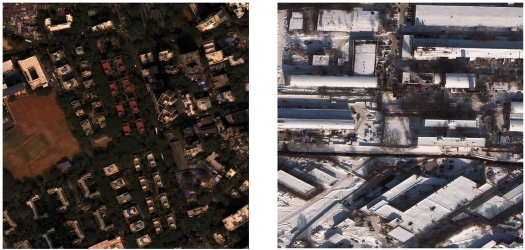
Both situations described above involve a shift between training data and the data encountered in practice. In a previous post we discussed the phenomenon of distribution shift through the lens of label shift. However, the change in satellite imagery induced by seasonal changes and the different distributions of ethnicities between facial training data and real life are examples of a different sort of distribution shift, covariate shift.

What is Covariate Shift?

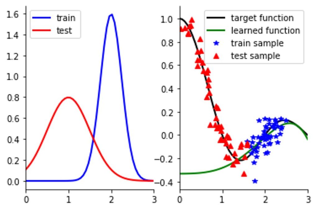
For many supervised machine learning applications such as image classification or automatic speech recognition (ASR) the data can be separated into observed variables that are inputs (e.g., images and waveforms) and predictions or target variables that are generally the output of trained models (e.g., labels and transcripts, respectively). Covariate shift is when the distribution of the inputs to the model is different from the training distribution (such as our previous snow example), without any change in the underlying mapping from inputs to outputs. The danger of covariate shift is that a model may not generalize to novel inputs that are different from those that it has been exposed to in training and will not perform accurately on.

There are number of solutions to covariate shift once it has been identified, including retraining the model on a new or reweighted training set, or excluding features from the input that are subject to change. However, before a machine learning practitioner can react to distribution shift, they have to first detect it. While many types of distribution shift can be obvious to human observers, some types of distribution shifts occur in subtle ways that are not obvious to humans, such as adversarial attacks. Furthermore, the large scale of many models means it is not feasible to require human identification of distribution shifts, and instead detection must be automated. To be useful, it is necessary that such an automatic system simultaneously be sensitive to harmful changes in the data distribution and at the same time not be triggered by the usual fluctuations in the data. One possible approach to automation is using well-calibrated statistical hypothesis testing for detecting distribution shift.

Applying statistical hypothesis testing to inputs like natural images or wave forms is difficult for several reasons. First the distributions of the training and testing inputs are very complex, lacking convenient mathematical descriptions. For example, assuming the data was normally distributed there are very efficient and simple tests for detecting changes. Second, unless we have a priori knowledge of what kind of differences to expect between the distributions, the detection methods have to be flexible enough to accommodate arbitrary types of shifts, as opposed to simpler tests like detecting a change in the mean. Fortunately two-sample tests, particularly nonparametric tests like the Kolmogorov-Smirnov or Kernel two-sample tests are particularly well suited for this purpose. Unfortunately, for high-dimensional inputs like images, these tests require infeasible amounts of samples. One solution is to use deep neural networks for dimensionality reduction before applying a statistical hypothesis test.

Detecting Covariate Shift in Speech Data

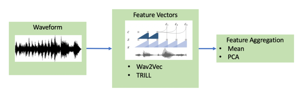
Many machine learning datasets used for speech applications such as automatic speech recognition (ASR) or speaker verification are based off speech audio recorded in ideal, close-up conditions. However, in realistic situations audio can be corrupted by environmental reverb or background noise. Speech recognition systems that are deployed in such environments should ideally be robust to changes in acoustic conditions or, failing that, automatically detect the shift and alert the user before suffering significant degradations in performance. In order to apply the aforementioned two-sample hypothesis testing framework on audio data, we use a two-stage preprocessing pipeline to transform the raw waveforms into fixed-length vectors.

1. We convert the waveforms into a sequence of feature vectors using one of two speech-embedding models:  Wav2Vec or TRILL. Both methods are self-supervised, and trained to produce general purpose representations of speech-audio, not just for speech recognition.
2. We aggregate the sequence of feature vectors into a single vector of the same dimension.  We have experimented with using the average vector, or first principal component of the set of vectors. More advanced techniques could include using RNN’s or Transformers to do this aggregation.

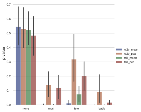
For a test case of our detection pipeline we utilize the VOiCES dataset. VOiCES is an audio corpus of fully transcribed speech recorded in a variety of realistic acoustic conditions, using a variety of microphones and background noises, with source audio derived from the Librispeech corpus. In another blog post we demonstrated that ASR models trained on Librispeech do not generalize well to VOiCES, even without added noise, despite using the same underlying speech data. To simulate the effect of changing acoustic conditions we assume the training data is drawn from VOiCES without any added background sound (denoted as ‘none’) and compute the p-value of the null hypothesis when the new data is drawn from VOiCES for different types of background sound. Because all acoustic conditions use the same subset of Librispeech for source audio, the only distribution shift that occurs will be in the acoustic conditions and not other factors such as transcript or speaker distributions.

Greater Impact

We have demonstrated that it is vital for any machine learning practitioner to know the limits of applicability for their models. When the model’s input data drifts far from that which it has been trained on, there are no guarantees on whether or not the model will maintain performance. While sophisticated statistical techniques can detect a broad range of shifts, methods that utilize domain knowledge are often an improvement. In the case of detecting a degradation in speech audio, classical techniques for estimating signal to noise ratio may be much more competitive. Building robust systems that safely operate in real-world conditions requires expertise in machine learning, as well as deep understanding of the problem domain. We invite others to try out our code for detecting acoustic shift.