Preface: SpaceNet LLC is a nonprofit organization dedicated to accelerating open source, artificial intelligence applied research for geospatial applications, specifically foundational mapping (i.e., building footprint & road network detection). SpaceNet is run in collaboration by co-founder and managing partner CosmiQ Works, co-founder and co-chair Maxar Technologies, and our partners including Amazon Web Services (AWS), Capella Space, Topcoder, IEEE GRSS, the National Geospatial-Intelligence Agency and Planet.

---

The recent SpaceNet 7 Challenge introduced the SpaceNet Change and Object Tracking (SCOT) metric, an evaluation metric for geospatial time series. In this post, we’ll use the results of SpaceNet 7 to explore how the metric acts with real-world data. We want to see whether the different parts of the metric really measure what they claim to measure. (Short answer: they do!)

The SpaceNet 7 dataset contains data for more than 100 distinct regions (“areas of interest” or AOIs) around the world. For each AOI, there is a deep stack of time series data, with one image per month for a period of about two years. The imagery is accompanied by building footprint labels that include an ID number for each building that persists from one month to the next, making it possible to track buildings over time and identify any new buildings each month. In the SpaceNet 7 Challenge, participants were asked to find the building footprints in each image and also to provide their own set of internally-consistent ID numbers, with the same building ideally getting the same ID number in every image where it appears.

Participants’ submissions were scored using the aforementioned SCOT metric. The metric compares a proposed set of footprints (with ID numbers) against ground truth, and it evaluates the proposal using two different terms: a tracking term and a change detection term. The tracking term measures how well the proposal tracks buildings from month to month. This term is basically an F1 score, but with a built-in penalty for inconsistent ID numbers. On the other hand, the change detection term measures how well the proposal identifies newly-built buildings, the most common change in this dataset. This term is also basically an F1 score, but it only uses building footprints making their chronological first appearance. Once the tracking and change detection terms are calculated for an AOI, their weighted harmonic mean gives the overall SCOT score for that AOI. To get the score for a collection of AOIs, a simple average of their individual SCOT scores is used. So that’s the math, but what does it mean in real life? Let’s find out.

Change versus Tracking

To explore the relationship between SCOT’s tracking and change detection terms in a model-independent way, we’ll use six different models: the five prize winners in SpaceNet 7 plus the SpaceNet 7 algorithmic baseline model. For each model, the SCOT metric is used to measure the model’s performance on each of the 21 AOIs in SpaceNet 7’s held-back private test set. That gives 126 comparison points (6 models x 21 AOIs), and Figure 1 shows the change score versus tracking score for each one.

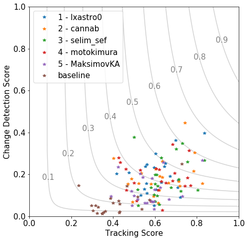
In Figure 1, the contour lines are lines of constant SCOT score. A careful inspection shows that the contours are not quite symmetric with respect to the two axes. That’s because the SCOT score is a weighted harmonic mean, and SpaceNet 7 used a non-equal weight (β=2, defined here) to prioritize the tracking score, thereby creating the observed asymmetry.

Turning our attention from the contour lines to the data itself, the first observation is evident: The median tracking score is much higher than the median change detection score, by a factor of about four. This may relate to the fact that a model can “recover” from a tracking error by being consistent in the subsequent time steps. But if a model misidentifies the time of construction, there are no opportunities for second chances.

The variation around the mean shows that, on average, higher tracking scores correlate with higher change detection scores. That’s not surprising — on the whole some models are better than others and some AOIs are easier than others, and both tracking and change detection can be expected to benefit from that. One difference among the models stands out in the plot: the five winning models noticeably outperform the baseline algorithm in both change and tracking. But even though the first-place model gets a SCOT score 33% higher than the fifth-place model, the data points from the prizewinners do not cluster by model. In other words, the variation among the AOIs for each model is not small compared to the variation among the prizewinning models’ averages. This same phenomenon was previously seen in, for example, SpaceNet 5.

Given the first-order correlation between change and tracking, do we really need both? When it comes to identifying the winner of SpaceNet 7, the differences do matter. Ranking the top five models by just the change detection score, instead of the complete SCOT score, would have swapped the order of 3rd and 4th place. The overall competition winner, lxastro0, rode to victory on the strength of a strong change detection score. If the winner had been decided by tracking alone, that submission would have instead come in 3rd. And the situation gets more interesting when we start looking at individual AOIs.

Regional Variation

Next, the data can be grouped by region, in other words, by AOI. We assign an arbitrary integer to each of the 21 AOIs in the private test set, and Figure 2 shows the performance of the five winning models, with each point labeled not by model but by AOI. To emphasize the distribution, a shaded polygon marks the convex hull of each AOI’s points. We leave out the baseline model here because its across-the-board lower scores obscure the inter-AOI variation we’re interested in.

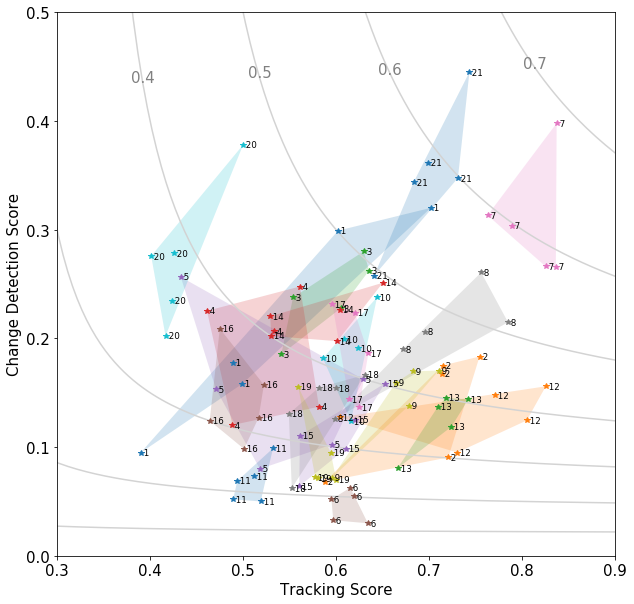
Despite a variety of neural network architectures and data processing approaches, all five models often produce tracking and change detection scores in the vicinity of other models for the same AOI. That suggests that the data’s departure from a strict one-to-one relationship between tracking score and change detection score is reflecting something intrinsic to the challenges posed by each AOI, rather than anything strictly model-dependent.

Figure 2 also gives a hint at where we can look next to get some clues about what’s going on. AOI 20 (in the upper left part of the figure) has consistently high change detection scores, despite having some of the lowest tracking scores. For AOI 12 (in the lower right), the opposite is true.

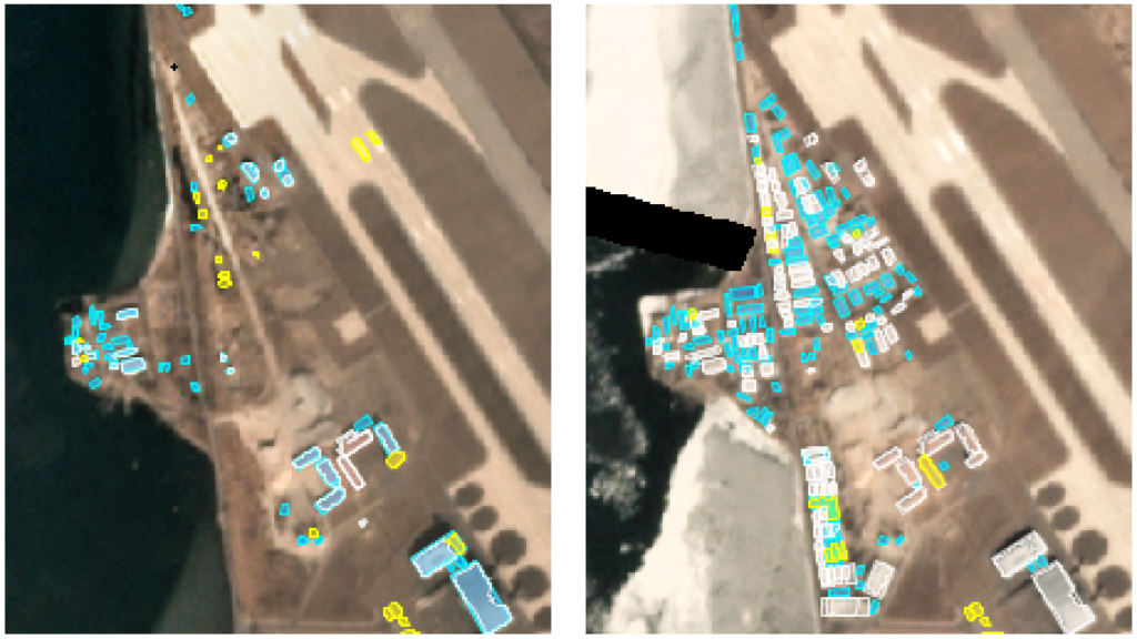
In the case of AOI 20, a closer inspection shows that many buildings fall into one of two extremes: those that are detected every month starting exactly when they were built, and those that are never detected at all. Figure 3 shows that immediately after construction, some buildings are detected while others aren’t. Over the following months, this distribution of true positives and false negatives persists in much the same way. As a result, the change detection score is almost as large as the tracking score, since so many of the tracked buildings get their time of first appearance correctly identified.

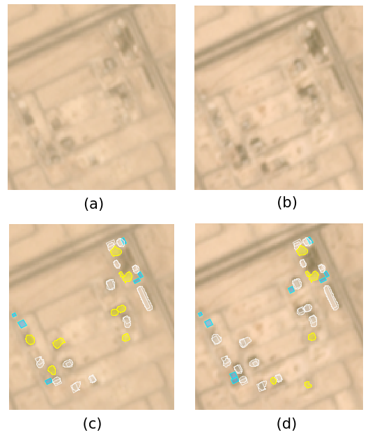
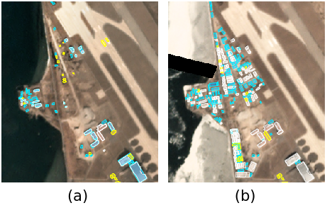
AOI 12, however, is a different story. In this region, the appearance of new buildings is frequently preceded by one or more months of what may be site preparation and/or construction activity. This often causes colors and textures that appear indistinguishable from those of a finished building. As a result, models frequently jump the gun and generate a building too early, as shown in Figure 4. (It is also possible that the ground truth labels are simply wrong, in which case the difficulty stems from this AOI’s labels, not its imagery.)

As these examples illustrate, difficulties related to the timing of construction most heavily drag down the change detection score, while difficulties that persist throughout the time series can weigh down the tracking score. The ability of the change detection score to identify time-sensitive problems around first appearance, and the corresponding ability of the tracking score to identify problems persisting in time, makes them complimentary measures of model success that both contribute to the holistic measure that is the SCOT metric.

This concludes our series analyzing the results of SpaceNet 7. Previous articles are here, here, and here, and look for the open-sourcing of the winning models coming soon.

---

This blog was originally published on The DownLinQ.