Where in the World, Part 2: A Deep Learning Model for Cross-view Image Geolocalization

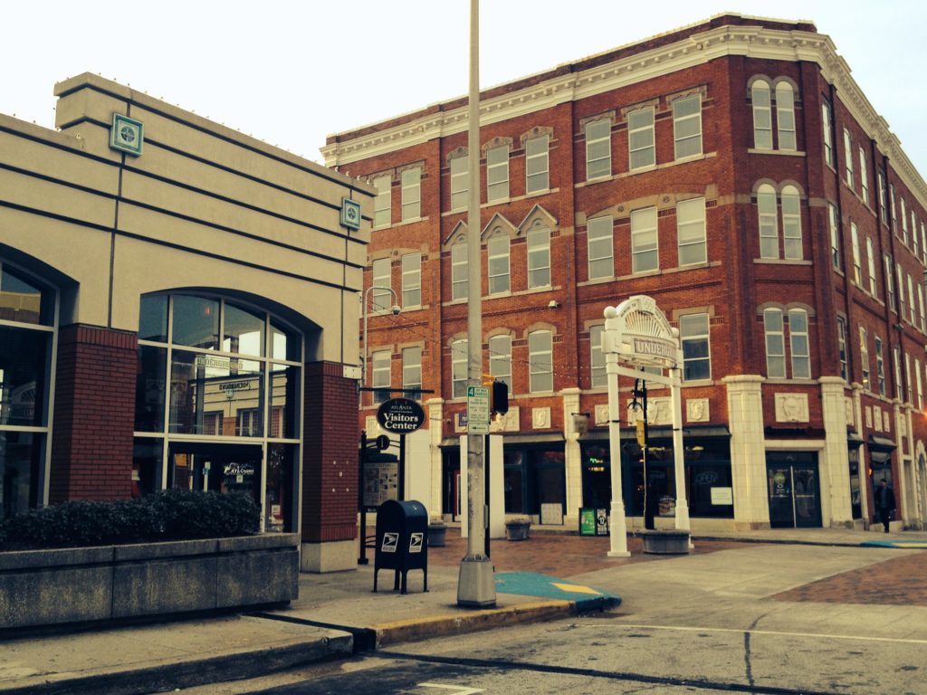
Cover image: CC BY Barbara Brannon

In the first post of this series, we introduced a new dataset for cross-view image geolocalization (CVIG), which is the task of finding a photograph’s geographic origin by comparing it to satellite images of candidate sites. The new dataset associates ground-level and overhead imagery, using ordinary photographs from thousands of amateur and professional photographers combined with high-resolution satellite imagery. With the dataset in place, we can now address the key question: how effectively can a deep learning model match a photograph to the satellite image of its location? To answer that, the next step for the Where in the World (WITW) project was to build such a model.

The Where in the World Model

Model Architecture

The Where in the World model is closely based on the state-of-the-art model of Shi et al. (2020), as introduced in their paper, “Where am I looking at? Joint Location and Orientation Estimation by Cross-View Matching.”

At the heart of this approach is a “twin” network architecture, also sometimes called a “Siamese” network architecture. In its simplest form, a twin network contains a convolutional neural network (CNN) for mapping overhead images into a feature space, and a second CNN for mapping ground-level images into the same feature space. The model is trained with a triplet loss function. Within each batch, the feature-space distance between each photo and its correct satellite image partner is reduced, while the distance between each photo and non-matching satellite images is increased. To take advantage of transfer learning, the two CNNs are both VGG16 networks with weights pretrained on ImageNet. During training, only the weights of the last six convolutional layers of each CNN are modified.

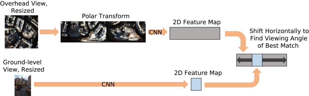
The twin network as described above has two limitations. First, a great deal of learning is required just to learn the basic spatial relationship between the ground and overhead views. Second, no consideration is made of the direction the photographer is facing when taking the ground-level picture, even though photos from the same spot can look completely different depending on what direction the camera’s pointed. To address both issues, the model architecture is enhanced as shown in Figure 1. First, the satellite imagery is converted into a crude sort of simulated panoramic view by applying a polar transformation. This polar-transformed image is then sent through one CNN, while the ground-level photo is sent through the other CNN (i.e., the “twin”). At this point, we have two feature maps, the outputs of the two CNNs. Each feature map shows the two-dimensional distribution of 16 learned features. The final step is to line up the feature maps and see how much the features differ. Since we don’t a priori know the direction the photographer was facing, we try every possible direction to find the one that leads to the lowest loss and use that. This method works whether the ground-level photo is a 360-degree panorama itself or a normal photo of smaller angular size like in Figure 1.

Model Implementation

While the WITW model hews closely to the techniques of Shi et al., the major differences concern implementation. Most importantly, the WITW model was built from the ground up in PyTorch. Compared to Shi et al.’s TensorFlow 1 codebase, the stylistic clarity and conciseness of PyTorch lends itself to modification and experimentation, examples of which will be seen below. Another difference is that our implementation automatically sets aside a subset of the training data (1000 randomly selected image pairs by default) for validation, allowing for validation-based early stopping.

The Where in the World model has been open-sourced under the Apache 2.0 license and is available in the WITW repository on GitHub. The same repo contains software tools used to create the dataset and to perform many of the analyses discussed in this and the following blog post.

Model Performance

To test the model, we used the image pairs from the Paris area of interest (AOI) as the test set. Image pairs for the 10 other cities were used as training data. This ensures a fair test by challenging the model with a city it has never seen before. Not only does that simulate a use case in a geographic area where training data is not available, it also prevents an artificial performance boost from having training and testing photos of the same places. In total, this split gives 106,185 image pairs for training and 58,270 for testing. Training takes about a day and a half on a Nvidia Titan Xp GPU.

The testing method is to look at each ground level photo in the test set. For each such ground-level photo, all the overhead images are ranked by how well they match it, as measured by how close they are in feature space. Two metrics are used to measure model performance. The first is “top-one,” which is the percentage of time that the correct overhead image is the closest match according to the model. The second is “top-percentile,” which is the percentage of time that the correct overhead image appears in the top percentile of ranked results. (We also calculated other metrics, including top-5, top-10, median rank, and mean rank, but for simplicity we’ll confine this discussion to just the previous two metrics.) Note that increasing the testing dataset size will tend to reduce the top-one metric, but not the top-percentile metric. Doubling the testing dataset size, for example, will roughly double the number of overhead images that are incorrectly ranked above the correct image. However, the number of images that make up the top percentile also doubles, and the two effects cancel out. That means the top-percentile metric can be used to compare results from different datasets, even if the testing datasets are not the same size.

On the CVUSA dataset, the WITW model performs similarly to Shi et al. In one trial, the WITW model’s top-one score of 82.53% and top-percentile score of 99.56% approach Shi et al.’s reported scores of 91.96% and 99.67%, respectively. If the CVUSA panoramas are cropped into random 70-degree-wide slices to create something a little more similar to ordinary photographs, then the WITW performance, again based on a single trial, was 6.10% for top-one and 60.91% for top-percentile, in comparison to 8.78% and 61.20%, respectively, reported by Shi et al.

These scores are numerically quite high. The CVUSA test set contains 8,884 image pairs, so getting a perfect match most of the time shows the capabilities of these models. But as discussed in the previous blog post, the well-aligned panoramas of CVUSA represent an artificially easy case compared to real-world applications with ordinary photographs, a situation which the WITW dataset was designed to approximate. To see the difference quantitatively, we trained and tested the WITW model using the WITW dataset. The result, averaging over three trials, was a top-percentile score of (3.92±0.15)% and a top-one score of only (0.0097±0.0055)%. Although the top-one scores cannot be directly compared because CVUSA and the WITW dataset have different-sized testing sets, it is valid to compare the top-percentile scores. The difference is striking: the same model architecture that scores above 99% on Street View panoramas scores around 4% on ordinary photographs.

This result shows that using CVIG to geolocate ordinary outdoor photographs is a far more difficult task than using CVIG to geolocate 360-degree panoramas of mostly rural roads produced for mapping services. That observation, which can get missed in investigations narrowly focused on the latter task, is made evident by using the WITW dataset.

Improving Model Performance

After developing the WITW model and using it with the WITW dataset to quantify the challenge of working with ordinary photographs, we considered different ways to improve the model’s performance. One issue is that the dataset contains photographs that aren’t applicable to CVIG, such as extreme close-up shots showing small details of the environment that could not possibly be spotted in a satellite photo. To address this, we produced a “filtered” version of the WITW dataset to increase the fraction of typical street scenes and reduce the fraction of irrelevant close-ups.

First, we hand-classified 500 ground-level photographs by whether they showed street scenes that could be amenable to CVIG. Each photograph was run through the Places model to produce a 467-element feature vector, containing 365 features related to scene classification and 102 features related to scene attributes. Although the Places model is designed to classify scenes, not predict whether something is a scene at all, we hypothesized that there were enough similarities between the tasks that this information would have diagnostic value.

Using 250 of the hand-classified photographs, an ensemble of 10 support vector machines (SVMs) was trained to classify images by whether they were usable scenes or not. The classifier was then tested using the other 250 hand-classified photos. The classifier had a precision of 80%, meaning that 80% of the images it identified as usable street scenes were cases where the human labeler agreed. Since only 54% of the original photos passed the cut, this was an improvement. At the same time, the classifier had a recall of 67%, meaning that only 1/3 of the usable street scenes were discarded in the process of producing this smaller, but higher-quality, subset of the dataset.

Training and testing the WITW model with this filtered WITW dataset improved the performance, raising the top-one score from (0.0097±0.0055)% to (0.012±0.003)% and raising the top-percentile score from (3.92±0.15)% to (4.40±0.15)%, as averaged over three trials. The increase in top-percentile score is statistically significant with a p-value of 0.015 in a two-sample T-test. As measured by top-percentile score, a model trained on the filtered dataset outperformed one trained on the original dataset when both were tested against the original test dataset, and the same was true when both were tested against the filtered test dataset. In short, this is a case where a smaller, higher-quality dataset gives better results than a larger, lower-quality dataset.

Other Performance Ideas

We also tried many potential improvements that in the end did not significantly increase model performance for the WITW model and dataset. In the interest of completeness, these are briefly described:

• In global mining, the members of each training batch are specially chosen to force the model to confront the most difficult-to-distinguish cases more often. The first half of each batch’s items is chosen at random, then the second half is made up of the nearest feature-space neighbors of the items in the first half.
• In the current model, the ground-level feature map is moved horizontally to find the viewing angle that best aligns with the polar transform’s feature map. One idea was to increase the height of the polar transform feature map so the ground-level feature map could also be moved vertically. The premise was that this might be a way for the model to better handle photos of objects at different distances.
• An idea that went in the opposite direction – towards greater simplicity instead of greater complexity – was to try using a simple twin network that did not explicitly take viewing angle into account. This was our baseline model, based on Liu & Li.
• We tried training the model on CVUSA and using the results as initial weights for training on the WITW dataset, on the grounds that the simpler CVUSA imagery might provide helpful feature learning as an intermediate step instead of going directly from ImageNet-trained weights to training on the WITW dataset.
• Some dataset changes were also explored. One simple change was using larger overhead imagery squares to include satellite imagery out to a greater distance.
• It is a known issue that Flickr photos often have imprecise geotags, so another idea was to deliberately offset the satellite images during training, to augment the data in a way that wasn’t much different from an already-present property of the dataset.
• The data from Paris shows an especially uneven geographic distribution, with two small sites, the Eiffel Tower and the Arc de Triomphe, that are highly over-represented. To see if this was having any unexpected effect on model testing performance, a testing data subset was tried that limited image pair geographic density. Another, simpler solution was to try removing the Mumbai AOI from training data and using it as the testing data instead of Paris. The geographic nonuniformity of the Paris data was not found to cause any particular problems.
• As discussed above, the Places model was used to increase the fraction of scene photos, as opposed to closeup photos, to make the dataset more suitable for CVIG. A different way to achieve the same outcome that was investigated was using the EfficientPS segmentation model on the ground-level photos and applying hand-engineered rules to the output. An example rule was to require the combined area of buildings, roads, and certain other scenery classes to exceed a given threshold.

Adding Semantic Input

Another approach that ultimately did not improve model performance, but warrants further discussion, was to add semantic information to the model’s input data. In this approach, we first identify which parts of each image show buildings or roads. Then, during training or testing, we feed that information into the model alongside the images themselves. The goal was to do some of the work in advance and thereby ease the model’s burden of having to learn to identify objects from RGB imagery alone. Buildings and roads were chosen because they are ubiquitous in the urban landscape, are readily visible from the ground as well as by satellite, and there exist automated tools to identify them in an image.

In the WITW dataset, the input images have three bands, corresponding to the amount of red, green, and blue in each pixel. To add some semantic information, these are augmented with two additional bands: one indicating if the pixel is likely to be showing part of a road, and one indicating if the pixel is likely to be showing part of a building. Figure 2 shows an example of what these extra bands look like.

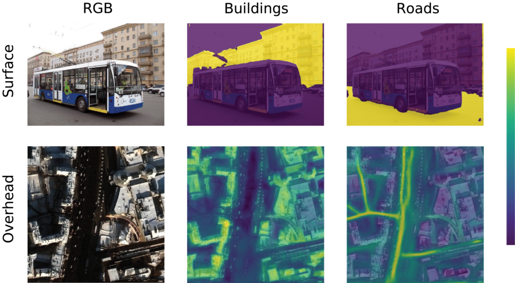
To identify roads and buildings in the ground-level photo, we again use the EfficientPS segmentation model. Although this model is capable of instance segmentation, here we just use it for semantic segmentation. Because the model assigns a single class to each pixel, the output for each semantic band (buildings and roads) is a binary mask.

For the overhead imagery, we identified buildings using the Solaris geospatial Python library previously developed by IQT Labs. This library includes a pretrained model for identifying building footprints in overhead imagery. Using the raw model output instead of applying a threshold gives us a continuous measure of how likely it is that a given pixel is part of a building, instead of a simple yes/no decision. In a similar approach, we trace out road centerlines using City-scale Road Extraction from Satellite Imagery (CRESI), also from IQT Labs. Once again, an included pretrained model is used to generate a continuously valued judgment about each pixel, but this time to evaluate which pixels are most likely near road centerlines.

To accommodate this five-channel input, the model had to be modified. The relevant dimension of the first convolutional layer was increased to allow five input bands, while still maintaining the pretrained weights for the RGB bands. Also, the number of layers that were updated during training was increased.

Surprisingly, adding this additional information reduced the model’s performance. In one trial, performance fell to a top-percentile score of 1.48%. Given that a model would achieve a top-percentile score of 1% by chance alone, that is a low score. One hypothesis is that the dataset isn’t large enough to learn to take advantage of this additional information. Instead of being helpful, the additional information might be providing more opportunities for overfitting on a too-small training dataset. This question of dataset size will be revisited in the next blog post.

Conclusion

By creating a new, flexible implementation of the state-of-the-art approach to CVIG, we can explore what is easy versus what is hard – and what works versus what doesn’t. We showed that geolocating unconstrained “in-the-wild” photographs is a far more difficult task than geolocating consistently aligned panoramas. In a wide-spanning study of model improvement ideas, we found it was possible to improve performance (by removing irrelevant image pairs from the training data), but seemingly promising approaches could often have the opposite effect. In the next post, we’ll analyze how the model performs under different circumstances, and in the process identify a factor that could lead to a substantial increase in the model’s performance.