

Preface: SpaceNet LLC is a nonprofit organization dedicated to accelerating open source, artificial intelligence applied research for geospatial applications, specifically foundational mapping (i.e., building footprint & road network detection). SpaceNet is run in collaboration by co-founder and managing partner CosmiQ Works, co-founder and co-chair Maxar Technologies, and our partners including Amazon Web Services (AWS), Capella Space, Topcoder, IEEE GRSS, the National Geospatial-Intelligence Agency and Planet.
The SpaceNet 7 Multi-temporal Urban Development Challenge yielded remarkable submissions from the winning competitors, as noted in our results announcement blog. In this post we will provide a deep dive into the winning algorithm, detailing the innovations that vastly improved upon the baseline model. We also note unexpected correlations between algorithmic performance and locale properties, namely: decreasing performance as resolution improves.
1. Baseline
The goal of SpaceNet 7 [1, 2] was to track building construction over time in moderate resolution Planet imagery over a deep time stack and dozens of areas of interest (AOIs) across six continents. CosmiQ Works constructed a baseline model to ascertain the feasibility of this task, which is illustrated in Figure 1.
2. Winning Approach
The winning team of lxastro0 (consisting of four Baidu engineers) improved upon the baseline approach in three key ways.
First, they swapped out the VGG16+U-Net architecture of the baseline with the far more advance HRNet, which maintains high-resolution representations through the whole network. Given the small size of the SpaceNet 7 buildings, mitigating the downsampling present in most architectures is highly desirable.
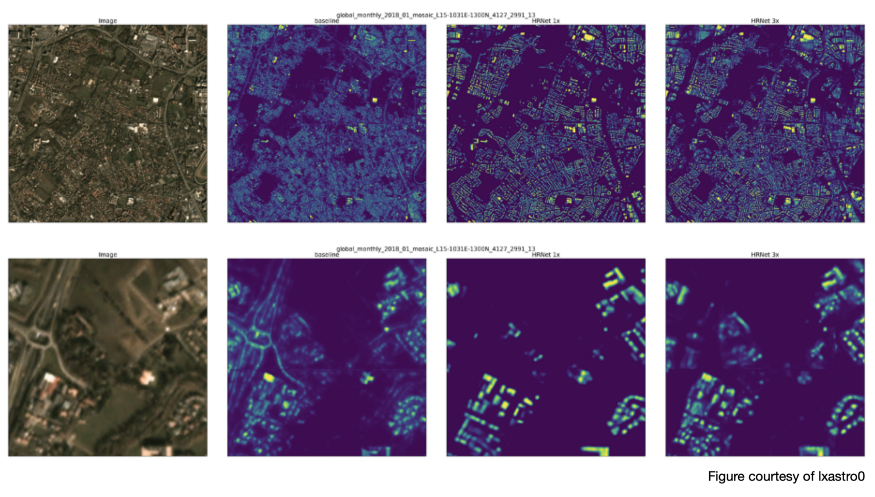
Second, the small size of objects if interest is further mitigated by upsampling the imagery 3× prior to ingestion into HRNet. The team experimented with both 2× and 3× upsampling, and found that 3× upsampling proved superior, see Figure 2.
Finally, and most crucially, the team adopted an elaborate post-processing scheme they term “temporal collapse” which we detail in the following section.
3. Temporal Collapse
In order to improve post-processing for SpaceNet 7, the winning team assumed:
(a) Buildings will not change after the first observation
(b) In the 3× scale, there is at least a one-pixel gap between buildings.
(c) There are three scenarios for all building candidates:
c.1. Always exists in all frames
c.2. Never exists in any frame
c.3. Appears at some frame k and persists thereafter
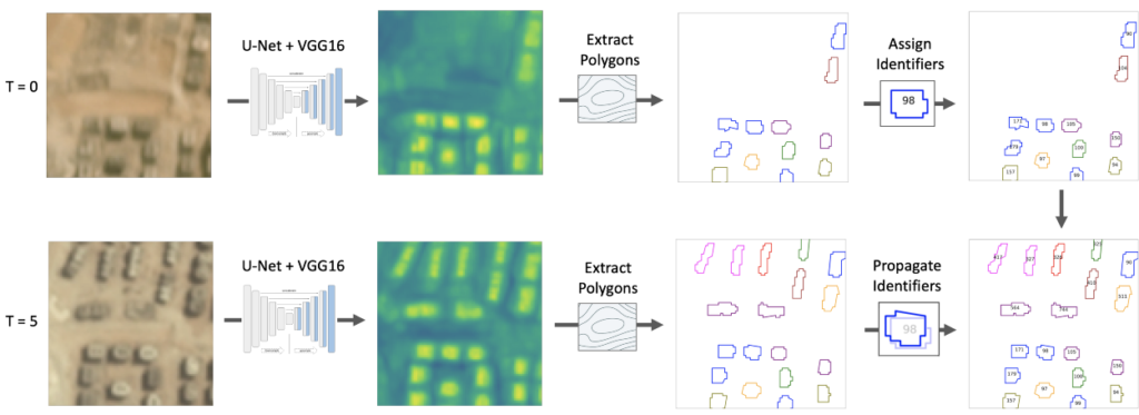
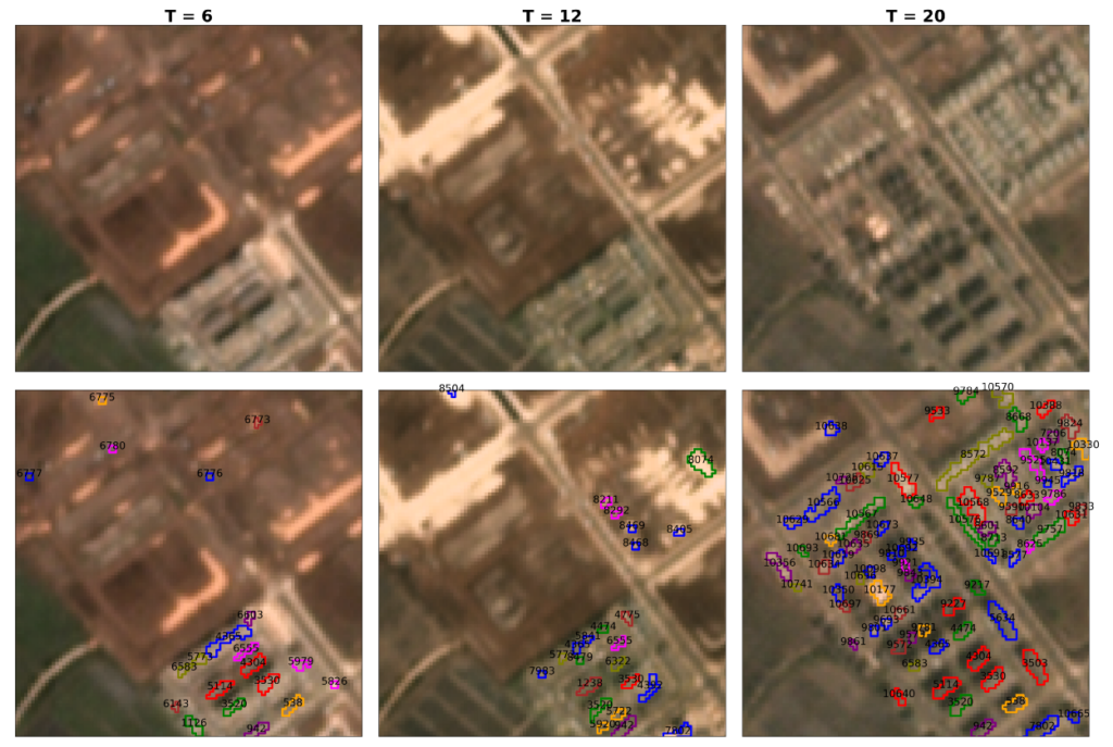
The data cube for each AOI can be treated as a video with a small (~24) number of frames. Since assumption (a) states that building boundaries are static over time, lxastro0 compresses the temporal dimension and predicts the spatial location of each building only once, as illustrated in Figure 3.
Building footprint boundaries are extracted from the collapsed mask using the watershed algorithm and an adaptive threshold, and taking into account assumption (b). This spatial collapse ensures that predicted building footprint boundaries remain the same throughout the time series.
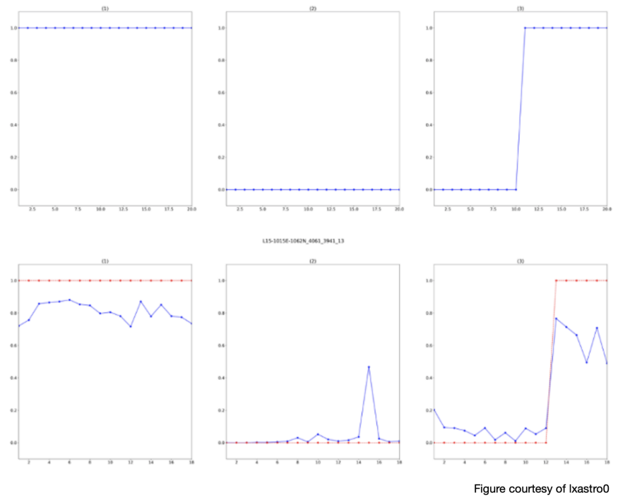
With the spatial location of each building now determined, the temporal origin must be computed. At each frame, and for each building, the winning team averaged the predicted probability values at each pixel inside the pre-determined building boundary. This mapping is then used to determine at which frame the building originated, as illustrated in Figure 4.
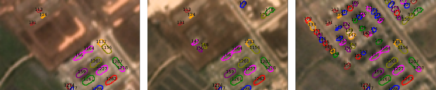
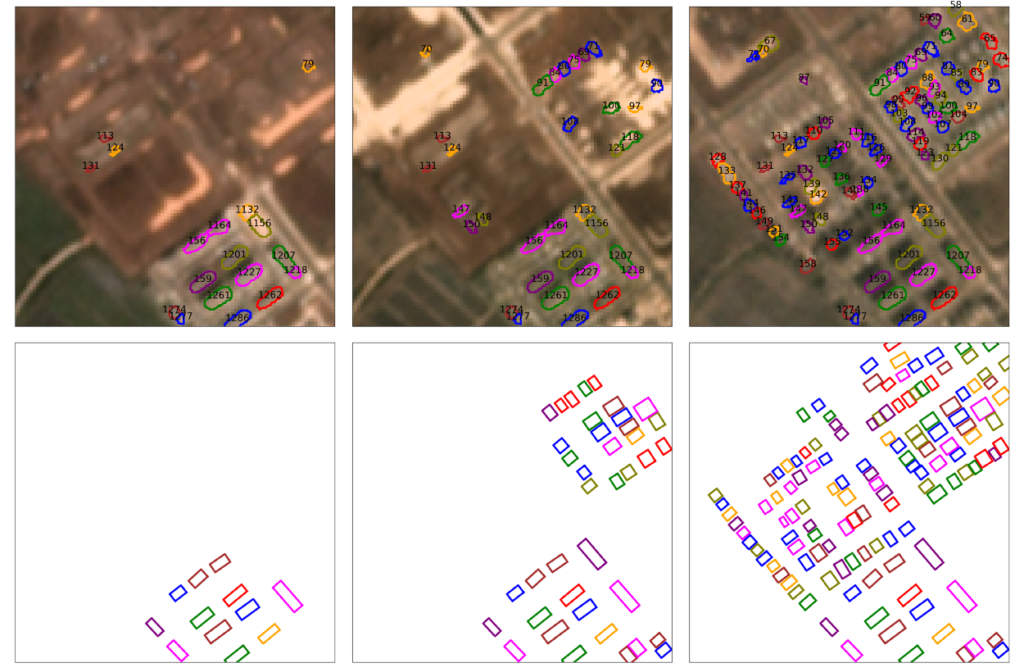
The techniques adopted by lxastro0 yield marked improvements over the baseline model in all metrics, but most importantly in the change detection term of the SpaceNet Change and Object Tracking (SCOT) metric. See Table 1 for quantitative improvements, and Figures 5 and 6 for qualitative examples. Further details on the winning algorithm (and all of the top-5 submissions) will be provided in the upcoming SpaceNet 7 model release blog post.

4. Analysis
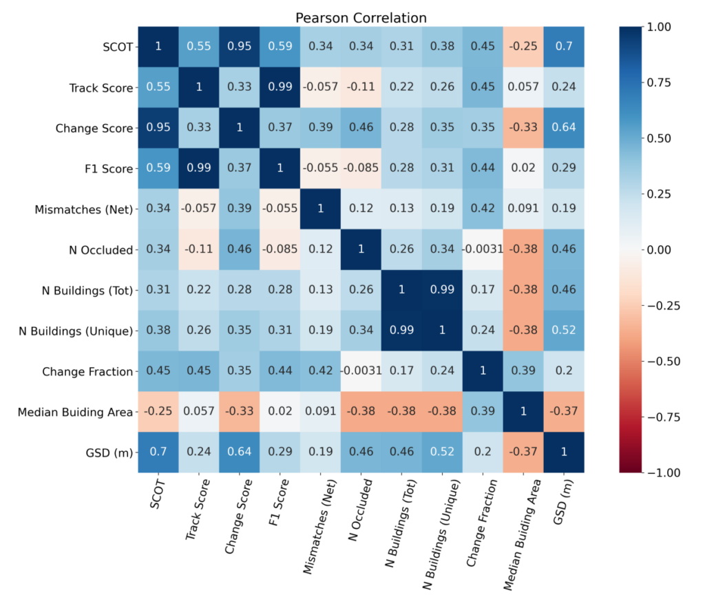
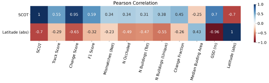
While Table 1 lists the aggregate performance of the winning model, there are a number of features of the dataset and scores that are worth exploring. Figure 7 displays the correlation between various variables across the AOIs for the winning submission. Most variables are positively correlated with the total SCOT score. Note the high correlation between SCOT and the Change Score; recall that SCOT is the weighted harmonic mean of the tracking term (Tracking Score) and the change detection term (Change Score), and since change detection is much harder this term ends up dominating.
5. Resolutions (Not the New Years Kind)
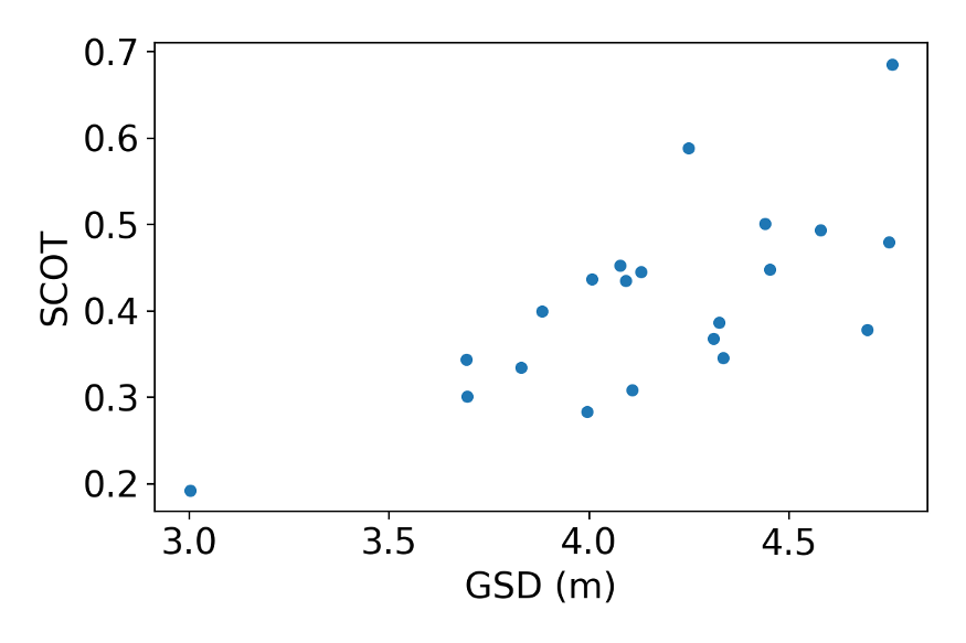
There are a number of intriguing correlations in Figure 7, but one particularly unexpected finding was the high (+0.7) correlation between ground sample distance (GSD), and SCOT. This correlation is even stronger than the correlation between SCOT and F1 score or SCOT and Track Score. Recall that GSD is the pixel size of the imagery, so a higher GSD corresponds to larger pixels and lower resolution. Furthermore, since all images are the same size in pixels (1024 × 1024), a larger GSD will cover more physical area, thereby increasing the density of buildings. Therefore, one would naively expect an inverse correlation between GSD and SCOT where increasing GSD leads to decreased SCOT, instead of the positive slope of Figure 8.
What is going on here? The ground resolved distance (GRD) is the same for all observations in the SpaceNet 7 dataset (GRD is the minimum distance such that two point targets can be detected as separate entities by the sensor). While the pixel size (GSD) changes, the resolving power is static, so it seems unlikely that the GSD — SCOT correlation implies causation.
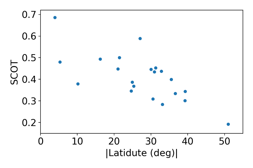
The processing of the SpaceNet 7 Planet imagery results in GSD ≈ 4.8m × Cos(Latitude). Therefore latitude (or more precisely, the absolute value of latitude) is negaively correlated with SCOT score. Building footprint tracking is apparently more difficult at higher latitudes, see Figure 9.
In Figure 10 we show correlations between various factors and both SCOT and latitude. Apparently, there are fewer buildings at higher latitudes, but few of the correlations of Figure 10 provide many clues as to why scores decrease with latitude. Yet the the high negative correlation between the change detection term (Change Score) and latitude is noteworthy.
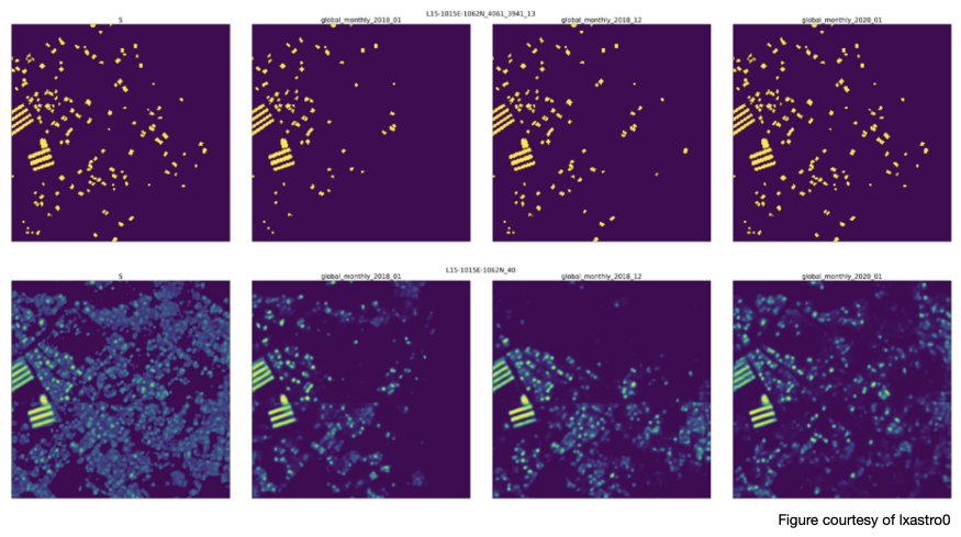
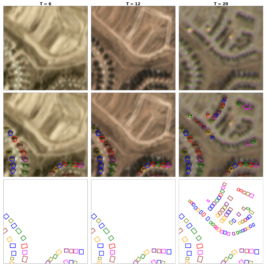
Evidently, identifying building change is significantly harder a higher latitudes. We leave conclusive proof of the reason for this phenomenon for a later date, but hypothesize that the reason is due to the greater seasonality and more shadows/worse illumination (due to more oblique sun angles) at higher latitudes. Figure 11 illustrates some of these effects. Note the greater shadows and seasonal change than in Figure 6. For reference, the change score for Figure 6 (latitude of 20 degrees) is 0.30, whereas the change score for Figure 10 (latitude of 40 degrees) is 0.09.
6. Conclusions
While all the top-5 winners of SpaceNet 7 Challenge managed impressive performance given the difficulties of tracking small buildings in medium resolution imagery, the winning team submitted by far the most creative, and rapid, proposal. By executing a “temporal collapse” and identifying temporal step functions in footprint probability, the winning team was able to vastly improve both object tracking and change detection performance.
Inspection of correlations between variables unearthed an expected decrease in performance with increasing resolution. Digging into this observation unearthed that the latent variable appears to be latitude, such that SCOT performance degrades at higher latitudes. We hypothesize that the greater lighting differences and seasonal foliage change of higher latitudes complicates change detection.
Apparently, ‘tis the season.
Thanks to Jesus Martinez Manso for assistance with Planet data collection specifics.