

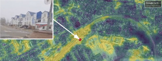
Cover image: Video frame via Twitter. Satellite imagery: Google, ©2022 Maxar Technologies.
The Russian invasion of Ukraine is playing out before the world on social media. The Economist has called Ukraine “the most wired country ever to be invaded,” and other outlets have discussed whether this amounts to the “First TikTok War.” Critical to verifying and interpreting a social media photo or video is geolocation, also called geolocalization, which means finding the place where the photo/video was recorded. Organizations that collect and geolocate social media from Ukraine include the Centre for Information Resilience, Bellingcat, The Washington Post’s visual forensics team, and The New York Times Visual Investigations team.
This post demonstrates how to find promising candidate locations for a photograph by using satellite imagery and deep learning. Geolocation is a painstaking process requiring a variety of skills, and the approach shown here cannot substitute for a trained human in pinpointing a photo’s origin. But this approach can sometimes suggest the most plausible areas to start the search, thereby making the human’s job a little less tedious. More broadly, this illustrates the strategy of applying open-source tools to open-source information, a combination with the potential to address problems across many domains.
How It’s Done
If you just want to see what the deep learning model can do, skip ahead to the next section. For the details of how it was created, here they are:
In a previous study of geolocation, we implemented a deep learning model based on a state-of-the-art approach to geolocating slices of 360-degree panoramas from mapping services like Google Street View. We determined how performance falls when using ordinary photographs instead of uniformly aligned imagery from mapping services. That insight motivated us to try a different method here, based on Workman et al., 2015, to better handle compositional variety (viewing angle, distance to subject, etc.) in social media photos.
To train a model to match photographs with satellite imagery, we need appropriate training data. Specifically, we need a dataset of image pairs, where each pair has a ground-level photo of an outdoor place accompanied by a satellite photo of the same location. We combine two such datasets. The first dataset is Workman’s original CVUSA dataset, which gets its ground-level photos from two sources: Google Street View and the photo-sharing website Flickr. The second dataset is our own “Where in the World” (WITW) dataset, with ground-level photos from Flickr. CVUSA’s overhead imagery comes from Bing Maps, and WITW’s overhead imagery is WorldView satellite imagery from SpaceNet. The CVUSA dataset is large, with ~1.6 million image pairs, mostly focused on rural areas. The WITW filtered dataset is smaller, with ~110,000 image pairs, and more focused on urban environments.
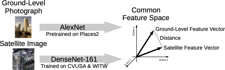
To build a model, we start with the pretrained models released by the creators of the Places2 dataset. These models classify photographs of places into 365 different scene categories (everything from airports to Zen gardens). We use the Places2 pretrained AlexNet model to generate a 365-element feature vector for each ground-level image. We then train a DenseNet-161 model to predict this feature vector from the corresponding overhead image. The initial values for the DenseNet model weights were taken from Places2’s pretrained DenseNet model, which produced better results than starting from random weights. We can see how well a photo matches a location by computing the Places2 feature vector for the photo, computing a feature vector for a patch of satellite imagery centered at the location with the newly trained model, and finding the distance between those feature vectors (smaller distance = better match). The satellite imagery patches fed into the model are 224 pixels on a side, and around 0.5m in resolution. Compared to our previous study, this approach improves performance on the WITW filtered test dataset, as measured by top-percentile score, from 4.4% to 5.7%. Figure 1 is a sketch of this approach.
Note that no ground-level imagery of Ukraine is required, except for the individual photo to be geolocated. Only satellite imagery of the search area is needed, which means this technique works just as well for places that (unlike Ukraine) have little to no coverage from Street View, Flickr, or other photo sources. All the training data used here comes from other places: CVUSA data is from the United States, and WITW data is from a selection of world cities, all outside Ukraine. Of those cities, the closest one to Ukraine, geographically, is Moscow.
Neighborhood-Scale Geolocation
We’ll use the model to narrow down possible locations for a photo within a small community.
Figure 2(a) shows a photograph of a destroyed railroad bridge in an otherwise open area. It was posted to Telegram and subsequently included in the Center for Information Resilience’s Eyes on Russia database. Figure 2(b) is a Google Earth satellite image of the small communities of Bucha and Irpin, which is where the photo is from. (The whitish polygons in the satellite image are places where the mosaic used imagery from a hazy day.) The deep learning model produces Figure 2(c), a heatmap showing the best matches in bright yellow. Each pixel of the heatmap is 10m wide.
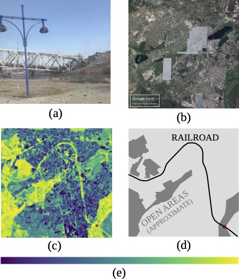
The actual origin of the photograph, marked with a red dot on the heatmap, was one of the best matches. Other open areas, which (like the photo) lack trees or buildings, also scored well. Most interestingly, the model responded to this photo of a railroad bridge by detecting the entire railroad line running through these communities, as shown by comparing Figures 2(c) and 2(d).
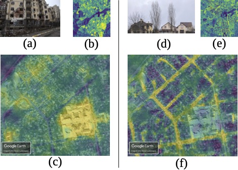
As another example, most photos of buildings generate similar-looking heatmaps, showing the built-up areas containing structures. However, there can be informative differences. Figure 3 shows the heatmaps from social media photos of a large apartment building and a pair of houses. On the scale of the whole 6km x 6km Bucha/Irpin area, both heatmaps highlight the areas with buildings. But zooming in on a detail shows that the first heatmap generates stronger matches in neighborhoods of large apartment buildings, while the second heatmap generates stronger matches along tree-lined residential streets.
National-Scale Geolocation
The same deep learning model used for finding potential matches in a small town can also be used to find potential matches on a much larger spatial scale, such as the entire 603,550 km2 of Ukraine.
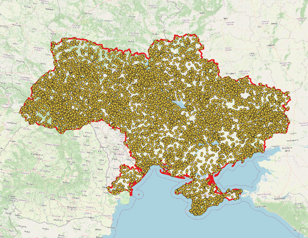
For the small-town case, we used a finely spaced grid of geographic points, calculating a feature vector for each one. To scale up, we instead use a random sample of points, exploiting the tendency of similar places to be near each other (“Tobler’s Law”). When selecting the random points, we want their geographic distribution to roughly follow the distribution of human activity. For example, densely packed cities should be more densely sampled than sparsely populated fields and forests. Therefore, we use randomly selected points from OpenStreetMap’s network of roads and paths. For each of 10,000 such points (Figure 4), we query the Bing Maps API for a satellite image from which to generate a feature vector.
To visualize the outcome, we divide the country into 25km-wide pixels. For a given ground-level photograph, we’ll define the feature-space distance of each pixel to be the distance of the best-matching feature vector within that pixel. On a scale from the worst-matching pixel distance to best-matching pixel distance, we’ll somewhat arbitrarily say any pixels in the top 10% of that range are “good candidates.”
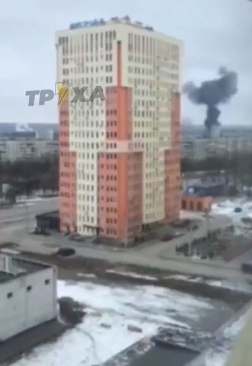
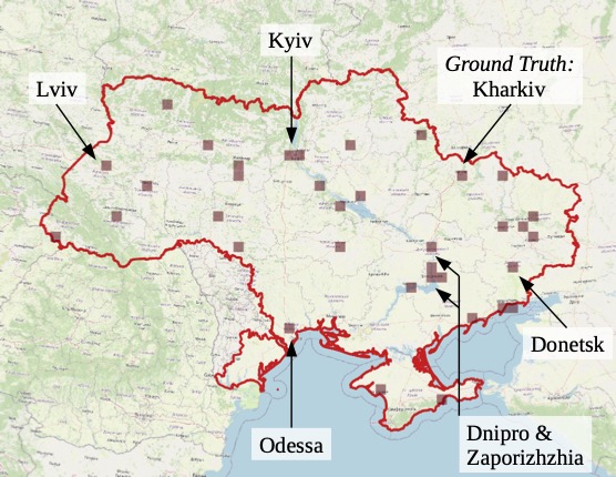
Having laid out the technique, let’s see some results. Figure 5 is a frame from a video posted on Twitter. Recorded in Kharkiv in February, it shows the aftermath of an explosion in the background, with a high-rise building in the foreground. Figure 6 shows a national map, with the model’s “good candidates” shaded brown. Out of more than a thousand pixels, the one covering Kharkiv is among the three dozen or so to reach that threshold. The false positives are perhaps the most interesting part of the story. By asking the model to geolocate a high-rise building, we have generated a map of the urbanized areas of Ukraine. As labeled on the map, the seven largest cities were all flagged as good candidates. Comparison to a map of Ukrainian cities shows that many of the other candidates are oblast (province) administrative centers or other major towns.
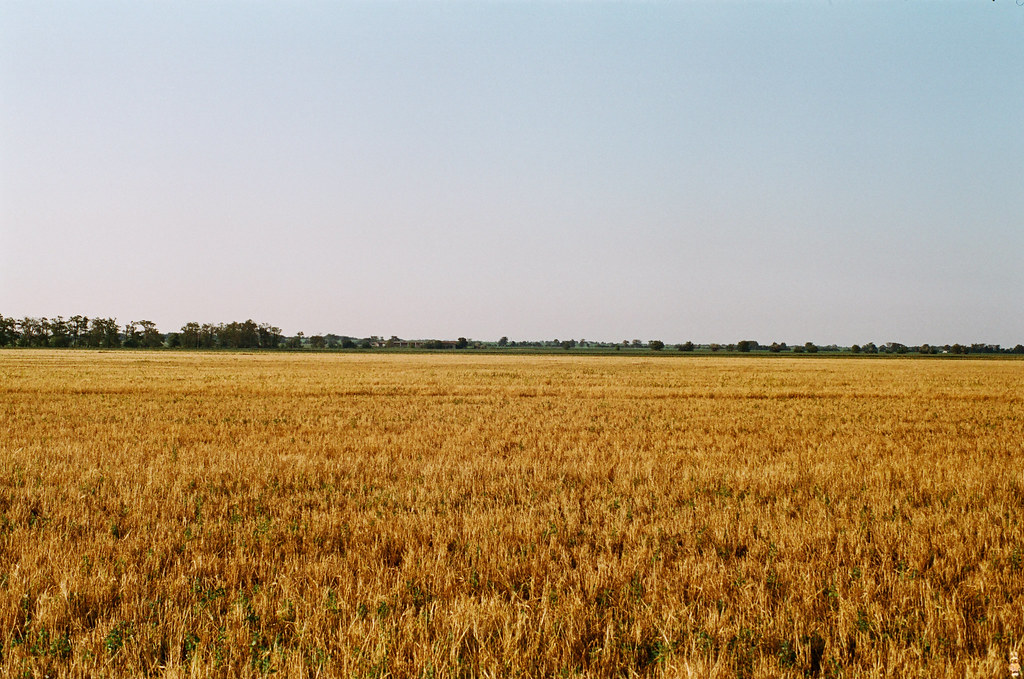
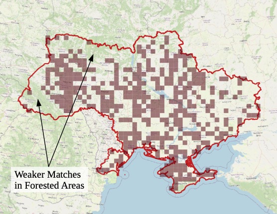
For another example, Figure 7 shows a photograph of a typical wheat field, taken in Ukraine a decade ago and posted to Flickr. Running it through the model gives Figure 8. Many good candidates can be found in this major agricultural country. And once again, the false positives tell a story – or rather, their absence does. The most-heavily forested parts of the country are shaded green in the OpenStreetMap base map used in Figure 8. These areas have noticeably fewer good candidates than other regions. The distribution of good candidates is also roughly consistent with a map of wheat production by oblast.
Interpretable Features
This analysis uses the Places2 model to map ground-level photos into a 365-dimensional feature space, and it uses another neural network to map satellite imagery into that same feature space. This Places2 feature space is interpretable, meaning that each component of a feature vector has a human-understandable meaning. Specifically, each component shows how much the photograph or satellite image seems to match a given scene class. In the following two examples, we use this information to build intuition for how the model behaves.
For the first example, the social media post linked here shows the same location in Kharkiv before and after buildings were destroyed. We can get a human-comprehensible description of what the model “sees” in each case by noting which feature vector components are largest. For the earlier picture, the model determines with 39% probability that it’s looking at a residential neighborhood. For the later picture, the model determines with 56% probability that it’s looking at desert sand, as it attempts to interpret an image that’s very different from typical Places2 training data. For large temporal changes like this, time differences between when the photo was taken and when the satellite imagery was collected can become important.
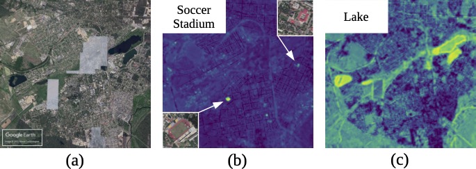
As a second example, we can search for Places2 scene classes without needing a ground-level photograph at all. For instance, one of the Places2 scene classes is soccer stadiums. By plotting the value of the corresponding feature vector component, we can make a heatmap for this scene type. Figure 9 shows such a heatmap for Bucha/Irpin, along with an analogous heatmap for lakes.
Discussion and Conclusions
In this project, we showed how to geolocate social media photos in a geopolitically important area, using a technique that doesn’t require any other ground-level photos from that area. Having an abundance of geolocated ground-level photos from an area opens up other options, but such data is not always available. Unlike some other approaches, the method used here does not require knowing/assuming the camera’s field of view, nor does it require a clear view of the horizon line.
The method used here is based on Workman et al., 2015. However, we go beyond that work in three ways:
- demonstrating that geolocation of ordinary photos is still possible with training data from outside the country,
- applying the method to a high-interest contemporary social media use case, and
- making technical improvements such as a newer neural network architecture and a globally usable way to select sample points for national-scale geolocation.
All this is made possible by leveraging publicly available and open-source datasets and software. Publicly available data used here includes the social media posts themselves, Google Earth, Google Street View (used in CVUSA), Bing Maps, Flickr, geolocated social media databases mentioned in the introduction, and boundary data from a non-governmental organization. That’s combined with open-source data from SpaceNet and OpenStreetMap. The analysis relies on open-source software, especially PyTorch, GDAL, QGIS, OSMnx, Places2, WITW, and our own open-source software repository on GitHub.
For this blog post, examples have been cherry-picked to show the model at its best. A model built on Places2 is most attuned to patterns of land use. For example, the model excels at the urban versus rural distinction, and our national-scale searches for skyscrapers and wheat fields benefit from that strength.
We speculate that certain improvements could lead to better performance across the board. First and foremost, simply acquiring more training data could improve performance on both the neighborhood and national scale. More sample points could improve national-scale performance. The approach could also benefit from retraining the Places2 models with additional labels, including simple features likely to be visible from overhead (e.g., “blue roof”). Finally, different satellite-based geolocation models could be used in tandem, such as the model used here alongside the Where in the World model. Expanding from a Ukraine-focused system to a worldwide system is largely a matter of scale, requiring sample feature vectors at many more points and, ideally, additional training data to further expand on the geographic variety of the SpaceNet-based Where in the World dataset.
Social media can be a valuable resource for understanding current events – if the information can be properly verified and contextualized. Geolocation is an important part of that process. By using deep learning and satellite imagery, it can be possible to identify candidate locations for social media photos and video frames. This approach has the potential to accelerate geolocation even when on-the-ground imagery is scarce, amplifying the ability to glean insights about the world from social media.